In a previous post, I explored building a supervised machine learning model using linear regression to predict the price of used cars. In this post, I will use supervised learning with classification to see if I can successfully build a model to predict whether a liability customer will buy a personal loan or not from a bank.
Before we dive in, I think it i important to distinguish between these two approaches in supervised learning. As a reminder, in linear regression, the algorithm learns to identify the linear relationship between input variables and output variables. The goal is to find the best-fitting line that describes the relationship between the input variables and the output variables. This line is determined by minimizing the sum of the squared differences between the predicted values and the actual values. During training, the algorithm is provided with a set of input variables and their corresponding output labels. The algorithm uses this data to learn the relationship between the input and output variables. Once the algorithm has learned this relationship, it can use it to make predictions on new, unseen data.
In classification, the algorithm learns to identify patterns in the input data and assign each input data point to one of several possible categories. The goal is to find a decision boundary that separates the different categories as well as possible. During training, the algorithm is provided with a set of input variables and their corresponding output labels, which represent the categories to which the input data points belong. The algorithm uses this data to learn the relationship between the input variables and the output labels, and to find the decision boundary that best separates the different categories. Once the algorithm has learned this relationship, it can use it to make predictions on new, unseen data.
Let’s get started.
Background and Context
AllLife Bank is a US bank that has a growing customer base. The majority of these customers are liability customers (depositors) with varying sizes of deposits. The number of customers who are also borrowers (asset customers) is quite small, and the bank is interested in expanding this base rapidly to bring in more loan business and in the process, earn more through the interest on loans. In particular, the management wants to explore ways of converting its liability customers to personal loan customers (while retaining them as depositors).
A campaign that the bank ran last year for liability customers showed a healthy conversion rate of over 9% success. This has encouraged the retail marketing department to devise campaigns with better target marketing to increase the success ratio.
We will attempt to build a model that will help the marketing department to identify the potential customers who have a higher probability of purchasing the loan.
Data Dictionary
- ID: Customer ID
- Age: Customer’s age in completed years
- Experience: #years of professional experience
- Income: Annual income of the customer (in thousand dollars)
- ZIP Code: Home Address ZIP code.
- Family: the Family size of the customer
- CCAvg: Average spending on credit cards per month (in thousand dollars)
- Education: Education Level. 1: Undergrad; 2: Graduate;3: Advanced/Professional
- Mortgage: Value of house mortgage if any. (in thousand dollars)
- Personal_Loan: Did this customer accept the personal loan offered in the last campaign?
- Securities_Account: Does the customer have securities account with the bank?
- CD_Account: Does the customer have a certificate of deposit (CD) account with the bank?
- Online: Do customers use internet banking facilities?
- CreditCard: Does the customer use a credit card issued by any other Bank (excluding All life Bank)?
Methodology
We will start by following the same methodology as we did in our linear regression model:
- Data Collection: Begin by collecting a dataset that contains the input features. This dataset will be split into a training set (used to train the model) and a testing set (used to evaluate the model’s performance).
- Data Preprocessing: Clean and preprocess the data, addressing any missing values or outliers, and scaling the input features to ensure that they are on the same scale.
- Model Training: Train the logistic regression model on the training dataset. This step involves finding the best-fitting line that minimizes the error between the actual and predicted purchase likelihood. Most programming languages, such as Python, R, or MATLAB, have built-in libraries that simplify this process.
- Model Evaluation: Evaluate the model’s performance on the testing dataset by comparing its predictions to the actual loan purchases. Common evaluation metrics for classification models include:
- Accuracy: The proportion of correctly classified instances to the total number of instances in the test set.
- Precision: The proportion of true positives (correctly classified positive instances) to the total number of predicted positives (instances classified as positive).
- Recall: The proportion of true positives to the total number of actual positives in the test set.
- F1 score: The harmonic mean of precision and recall, which provides a balance between the two measures.
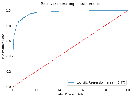
- Area under the receiver operating characteristic curve (AUC-ROC): A measure of the performance of the algorithm at different threshold levels for classification. The AUC-ROC curve plots the true positive rate (recall) against the false positive rate (1-specificity) for different threshold levels.
- Confusion matrix: A table that summarizes the actual and predicted classifications for each class. It provides information on the true positives, true negatives, false positives, and false negatives.
- Model Optimization: If the model’s performance is unsatisfactory, consider feature engineering, adding more data, or using regularization techniques to improve the model’s accuracy.
The dataset used to build this model can be found by visiting my GitHub page.
Data Collection
We will start by importing all our required Python libraries:
#Import NumPy
import numpy as np

#Import Pandas
import pandas as pd
pd.set_option('mode.chained_assignment', None)
pd.set_option("display.max_columns", None)
pd.set_option("display.max_rows", 200)

#Import matplotlib
import matplotlib.pyplot as plt
%matplotlib inline

#Import Seaborn
import seaborn as sns

#Import sklearn libraries
from sklearn.linear_model import LogisticRegression
from sklearn.model_selection import train_test_split
from sklearn.model_selection import GridSearchCV
from sklearn.tree import DecisionTreeClassifier
from sklearn import tree
from sklearn.metrics import (
    f1_score,
    accuracy_score,
    recall_score,
    precision_score,
    confusion_matrix,
    roc_auc_score,
    plot_confusion_matrix,
    precision_recall_curve,
    roc_curve,
)

#Beautify Python code
%reload_ext nb_black

#Import warnings
import warnings
warnings.filterwarnings("ignore")

#Import Metrics
from sklearn import metrics
Now we will import the dataset. For this project, I used Google Colab.
#mount and connect Google Drive
from google.colab import drive
drive.mount('/content/drive')

#Import dataset "used_cars_data.csv"
data = pd.read_csv('/content/drive/My Drive/Colab Notebooks/Loan_Modeling.csv')
Data Preprocessing, EDA, and Univariate/Multivariate Analysis
As always, we will start by reviewing the data:
#Return random data sample
data.sample(10)
Next, we will evaluate how may rows and columns are in the dataset:
#Number of rows and columns
print(f'Number of rows: {data.shape[0]} and Number of columns: {data.shape[1]}')
As we can see, there are 5,000 rows and 14 columns.
Next, we will review the datatypes:
#Data type review
data.info()
It does not appear that there is any missing data in the dataset. We can confirm by running:
#Confirming no data is missing
data.isnull().sum()
Let’s see if there is any duplicated data:
#Check for duplicates
data.duplicated().sum()
There is no duplicated data identified. Additionally, the ID column does not offer any added value so we will drop this column.
#Drop ID column
data.drop(['ID'], axis=1, inplace=True)
data.reset_index(inplace=True, drop=True)
Next, we will review the statistical analysis:
#Statistical summary of dataset
data.describe().T
Here is what we found:
Age
- Mean: 45.3
- Minimum Age: 23
- Maximum Age: 67
Experience
- Mean: 20.1
- Minimum Experience: -3
- Maximum Experience: 43
(We will address the negative values below)
Income
- Mean: 73.8
- Minimum Income: 8
- Maximum Income: 224
Family
- Mean: 2.4
- Minimum Family: 1
- Maximum Family: 4
CC Avg
- Mean: 1.9
- Minimum CC Avg: 0
- Maximum CC Avg: 10
Education
- Mean: 1.9
- Minimum Education: 1
- Maximum Age: 3
Mortgage
- Mean: 56.5
- Minimum Mortgage: 0
- Maximum Mortgage: 635
Next. we will review the unique values in the dataset:
#Review unique values
pd.DataFrame(data.nunique())
Zip codes seem to have the most unique values. Since we are dealing with logistic regression which does classifications based on categories, we will want to convert the zip codes into something we can categorize. Since city would most likely return the same number of unique values, we will convert the zip codes to be based on county. This is a mush more macro approach and should reduce the number of unique values in the dataset. This is also a much better approach as all of the zip codes appear to be located in the same state so using the state instead of zip code would not offer much value.
#Install the Python zipcode library
!pip install zipcodes
First, we create a list of all the unique values for ZIPCode which will enable us to create an iterative for loop. We will then store these in a dictionary as Zip Code mapped to the county. We will convert the stored values to a string. If the county conversion cannot be identified, we will simply keep the zip code and evaluate the results.
#Import the zipcodes Python package
import zipcodes

#Create a list of the zip codes in the dataset based on these unique values
zip_list = data.ZIPCode.unique()
zipcode_dictionary = {}

for zip in zip_list:
    zip_to_county = zipcodes.matching(zip.astype('str'))
    if len(zip_to_county)==1:

    #Get the county from the zipcodes package
        county = zip_to_county[0].get('county')

    else:
        county = zip
    zipcode_dictionary.update({zip:county})

#Return the dictionary
zipcode_dictionary
The following zip codes were not mapped to the county:
- 92634
- 92717
- 93077
- 96651
We will drop these rows.
#Drop all rows with 92634 zip code
data = data[data["ZIPCode"] != 92634]

#Drop all rows with 92717 zip code
data = data[data["ZIPCode"] != 92717]

#Drop all rows with 93077 zip code
data = data[data["ZIPCode"] != 93077]

#Drop all rows with 96651 zip code
data = data[data["ZIPCode"] != 96651]
Let’s review the shape of the data now:
#Review the shape of the data
data.shape
The data shape has now been reduced by (1) column after dropping the ID column and (44) rows by eliminating zip codes that could not be mapped to a county. We now need to map these counties to the dataset by using the map function. According to the map function “returns a list of the results after applying the given function to each item of a given iterable.”
Next, we will create a new column called County that maps the zip codes in the dataset to the new feature, counties.
#Create new column county that maps the zip codes accordingly
data['County'] = data['ZIPCode'].map(zipcode_dictionary)
We will now convert the newly created county column to a categorical datatype.
#Convert the county column to a category
data['County'].astype('category')
To review the counties by count:
#Value counts by county
data['County'].value_counts()
The top five counties where customers reside are as follows:
- Los Angeles County: 1095
- San Diego County: 568
- Santa Clara County: 563
- Alameda County: 500
- Orange County: 339
It was observed above that there were some negative values in the experience column above that we need to address. We can do a number of things here. We can impute using a measure of central tendency, we could drop the rows, we can replace these with zeros, or we can use the absolute value function. Let’s first understand the impact before we determine which strategy would be best.
#Identify all the rows with negative values for experience
data[data['Experience'] < 0].value_counts().sum()
There are 51 rows with negative values for the experience column. Since it is impossible to have a negative number of years of experience and we do not know if this was a clerical error, we are going to replace those values with zeros. We could also use the absolute value, but we chose to make them 0.
#Replace negative values with zeros
data.loc[data['Experience']<0,'Experience'] = 0
Let’s take a visual look at the continuous data in the dataset:
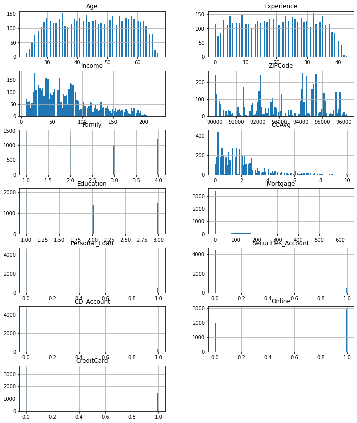
As we move to univariate analysis, I decided to create a function to make representing this data graphically easier.
#Create a function for univariate analysis (code used from Class Module)
def histogram_boxplot(data, feature, figsize=(12, 7), kde=False, bins=None):
    f2, (ax_box2, ax_hist2) = plt.subplots(
        nrows=2,
        sharex=True,
        gridspec_kw={"height_ratios": (0.25, 0.75)},
        figsize=figsize,
    )
    sns.boxplot(
        data=data, x=feature, ax=ax_box2, showmeans=True, color="violet"
    )
    sns.histplot(
        data=data, x=feature, kde=kde, ax=ax_hist2, bins=bins, palette="winter"
    ) if bins else sns.histplot(
        data=data, x=feature, kde=kde, ax=ax_hist2
    )
    ax_hist2.axvline(
        data[feature].mean(), color="green", linestyle="--"
    )
    ax_hist2.axvline(
        data[feature].median(), color="black", linestyle="-"
    )
Additionally, I built a function to help identify outliers that exist in our dataset.
#Create function for outlier identification
def feature_outliers(feature: str, data = data):
    Q1 = data[feature].quantile(0.25)
    Q3 = data[feature].quantile(0.75)
    IQR = Q3 - Q1
    return data[((data[feature] < (Q1 - 1.5 * IQR)) | (data[feature] > (Q3 + 1.5 * IQR)))]
Evaluating the age feature, we see the age feature looks relatively normal and even.
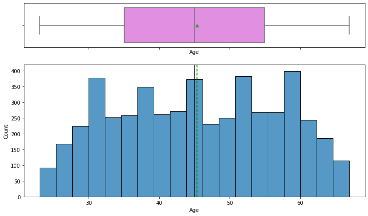
The mean and median ages are approximately 45 years old:
#Mean of age
print(data['Age'].mean())

#Median of age
print(data['Age'].median())
We also identified that there were no outliers in the age feature.
#Evaluate outliers
age_outliers = feature_outliers('Age')
age_outliers.sort_values(by = 'Age', ascending = False)
age_outliers
Looking at the education feature, we see that the mean and median number of years respectively is 1.88 and 2.0 years.
#Mean of education
print(data['Education'].mean())

#Median of education
print(data['Education'].median())
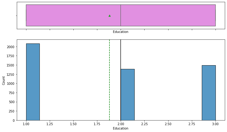
We will also convert this feature to categorical datatype:
#Convert Education columns to category
data[‘Education’] = data[‘Education’].astype(‘category’, errors = ‘raise’)
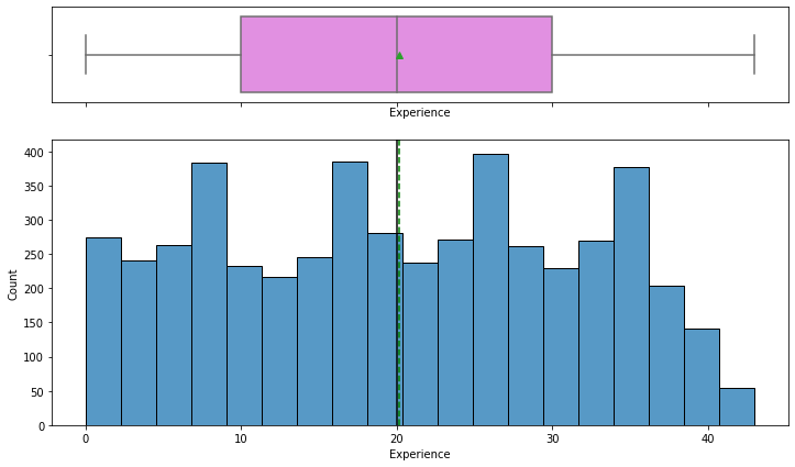
Next, we will review the experience feature. The mean experience is 20.1 and the median is 20. This data looks relatively normal. Additionally, there were no outliers.
#Mean of experience
print(data['Experience'].mean())

#Median of experience
print(data['Experience'].median())

#Evaluate outliers
experience_outliers = feature_outliers('Experience')
experience_outliers.sort_values(by = 'Experience', ascending = False)
experience_outliers
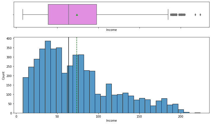
The data for the income feature is right skewed.There is approximately $10,000 difference between the mean and median income. Additionally, there are 96 outliers for the income feature. We will not change these as these customers may be in the market for a personal loan.
#Mean of income
print(data['Income'].mean())

#Mean of income
print(data['Income'].median())

#Evaluate outliers
income_outliers = feature_outliers('Income')
income_outliers.sort_values(by = 'Income', ascending = False)
income_outliers.head()
income_outliers.value_counts().sum()
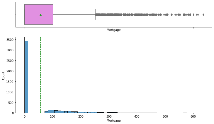
There are 3,435 customers in the dataset that do not report having a mortgage. There are 289 outliers for the mortgage feature. Again, we will leave these as is.
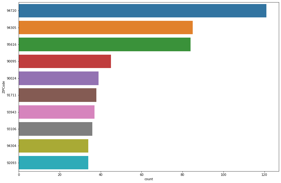
Let’s also evaluate the top 10 zip codes of where our customers reside who do not have a mortgage.
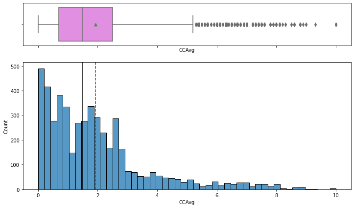
We also observed the mean for the CCAvg feature is 1.9 and the median is 1.5. There were also 320 outliers identified for the CCAvg feature. We will leave this as some customers may apply for personal loans for debt consolidation.
The mean family size is 2.4 and the median is 2.0. We will convert the family column to a categorical datatype.
#Mean of family
print(data['Family'].mean())

#Median of experience
print(data['Family'].median())

#Convert family columns to category
data['Family'].astype('category', errors = 'raise')

The top three counties are:
- Los Angeles County
- San Diego County
- Santa Clara County

We will convert this column to a categorical datatype and drop the Zip Code column.
#Convert County columns to category
data['County'] = data['County'].astype('category', errors = 'raise')

#Drop ZIPCode column
data.drop(['ZIPCode'], axis=1, inplace=True)
data.reset_index(inplace=True, drop=True)
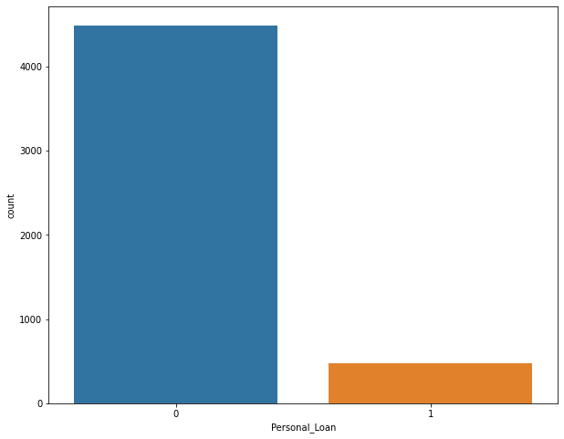
The data showed that only 10.63% of customers in the dataset have a personal loan. Our next step is to convert this feature into a category.
#Percentage of customers with personal loans
percentage = pd.DataFrame(data['Personal_Loan'].value_counts(ascending=False))
took_personal_loan = (percentage.loc[1]/percentage.loc[0] * 100).round(2)
print(f'{took_personal_loan[0]}% of customers have a personal loan.')
#Convert Personal_Loancolumns to category
data['Personal_Loan'] = data['Personal_Loan'].astype('category', errors = 'raise')
We observed that 11.62% of customers have security accounts. We will convert the security accounts to a categorical datatype.
#Percentage of customers with personal loans
percentage = pd.DataFrame(data['Personal_Loan'].value_counts(ascending=False))
took_personal_loan = (percentage.loc[1]/percentage.loc[0] * 100).round(2)
print(f'{took_personal_loan[0]}% of customers have a personal loan.')
There are a few other features we could have conducted our univariate analysis on, however for the sake of brevity, here is the main findings:
- The mean age is 45.3 years old and the median age is 45
- The mean experience is 20.1 and the median age is 20
- The mean income is approximately
- 64,000 per year. There is approximately $10,000 difference between the mean and median.
- The mean CCAvg is 1.9 and the median is 1.5
- 10.63% of customers have a personal loan
- 67.54% of customers use online banking
- 11.62% of customers have security accounts
- 6.48% of customers have a CD account
- 41.56% of customers have a credit card account
- The top three counties are Los Angeles County, San Diego County, and Santa Clara County
- The mean education is 1.9 and the median is 2.0
We will now create a function to assist in our bivariate analysis:
#Function for Multivariate analysis (code taken from class notes)

def stacked_barplot(data, predictor, target):
    count = data[predictor].nunique()
    sorter = data[target].value_counts().index[-1]
    tab1 = pd.crosstab(data[predictor], data[target], margins=True).sort_values(
        by=sorter, ascending=False
    )
    print(tab1)
    print("-" * 120)
    tab = pd.crosstab(data[predictor], data[target], normalize="index").sort_values(
        by=sorter, ascending=False
    )
    tab.plot(kind="bar", stacked=True, figsize=(count + 5, 6))
    plt.legend(
        loc="lower left", frameon=False,
        plt.legend(loc=“upper left”, bbox_to_anchor=(1, 1))

        plt.show()
    )
Now that we have the function created, let’s look at the breakdown of those customers with personal loans broken down by family size.
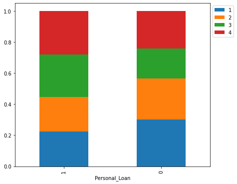
We see that the families with 3 kids are the largest demographic with personal loans. Another interesting fact that we identified in our bivariate analysis is that more people in the 60+ age group took the personal loan than those who didn’t. Most people who took the personal loan are between the ages of 30-60.

Below is a breakdown of the continuous values in the dataset in a pair plot:
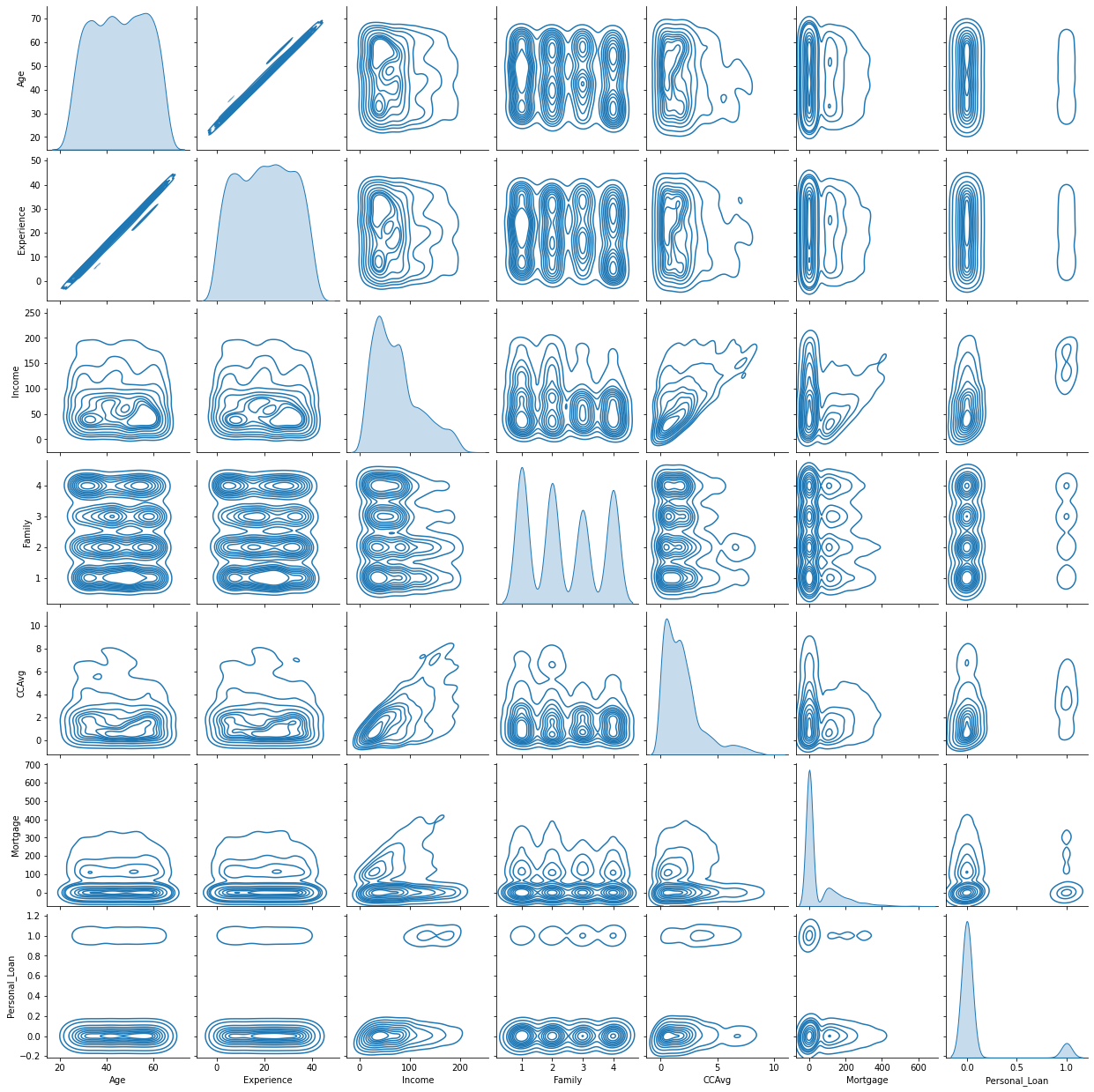
This helped us identify that the experience column does not appear to offer much value in terms of building the models so we will drop this column. Since age and experience go are so heavily correlated, we do not need this column. We will drop experience and keep age.
#Drop Experience column
data.drop(['Experience'], axis=1, inplace=True)
data.reset_index(inplace=True, drop=True)
Below is a heat map of the numerical representations of the correlation:

Model Building
Now that our data analysis is completed, we will start building some models. We will first start with using a standard logistic regression model as our baseline to see if we can improve upon the results in iterations.
The first step is to make a copy of our original dataset.
#Copy dataset for logistic regression model
data_lr = data.copy()
Now that we are using a clean dataset, we can start building our logistic regression model. To begin, we will drop the dependent variable and use the same one-hot encoding technique we used in our linear regression model. W will encode the county, family, and education features.
Model using sklearn
#Beginning building Logistic Regression Model
x = data_lr.drop(['Personal_Loan'], axis=1)
y = data_lr['Personal_Loan']

#Use OneHot Encoding on county, family, and education
oneHotCols=['County','Education', 'Family']
x = pd.get_dummies(x, columns = oneHotCols, drop_first = True)
Next, we will split our dataset into training and testing data respectively.
# splitting in training and test set
x_train, x_test, y_train, y_test = train_test_split(x, y, test_size=0.3, random_state=1)
We now have 3,476 rows in our training data and 1,490 rows in our testing dataset. Now that it is split, we can effectively fit the model using the libliner solver, predict on the test data, and evaluate the coefficients.
#Build the model
model = LogisticRegression(solver="liblinear", random_state=1)
lg = model.fit(x_train, y_train)

#predicting on test
y_predict = model.predict(x_test)

#Evaluate the coefficients
coef_df = pd.DataFrame(
    np.append(lg.coef_, lg.intercept_),
    index=x_train.columns.tolist() + ["Intercept"],
    columns=["Coefficients"],
)
coef_df.T
What we notice here is that the coefficients of age, securities account, online, credit card, El Dorado County, Fresno County, Humboldt County, Imperial County, Lake County, Los Angeles County, Mendocino County, Merced County, Monterey County, Placer County, Riverside County, Sacramento County, San Benito County, San Bernardino County, San Diego County, San Francisco County, San Joaquin County, San Luis Obispo County, San Mateo County, Santa Barbara County, Santa Cruz County, Shasta County, Siskiyou County, Stanislaus County, Trinity County, Tuolumne County, and Family_2 are negative and an increase in these will lead to decrease in chances they purchase a personal loan.
Let’s evaluate the results on the training dataset:

- True Negatives (TN): Correctly predicted that they do not have personal loan (3,213)
- True Positives (TP): Correctly predicted that they have personal loan (213)
- False Positives (FP): Incorrectly predicted that they have a personal loan (24 falsely predict positive Type I error)
- False Negatives (FN): Incorrectly predicted that they don’t have a personal loan (116 falsely predict negative Type II error)
In evaluating the training performance, we see the accuracy score really well, but the recall is pretty low here.
#Evaluate metrics on the Training Data (Taken from class module)
log_reg_model_train_perf = model_performance_classification_sklearn_with_threshold(lg, x_train, y_train)
print("Training performance:")
log_reg_model_train_perf
| Accuracy | Recall | Precision | F1 | |
| 0.959724 | 0.647416 | 0.898734 | 0.75265 |
The coefficients of the logistic regression model are in terms of log(odd), to find the odds we have to take the exponential of the coefficients. Therefore, odds = exp(b). The percentage change in odds is given as odds = (exp(b) – 1) * 100
#Converting coefficients to odds
odds = np.exp(lg.coef_[0])

#Finding the percentage change
perc_change_odds = (np.exp(lg.coef_[0]) - 1) * 100

#Removing limit from number of columns to display
pd.set_option("display.max_columns", None)

# Adding the odds to a dataframe
pd.DataFrame({"Odds": odds, "Change_odd%": perc_change_odds}, index=x_train.columns).T
- Age: A 1 unit change in Age will decrease the odds of a person buying a personal loan by 0.98 times or a 1.58% decrease in odds of having purchased a personal loan.
- Income: a 1 unit change in the Income will increase the odds of a person having purchased a personal loan by 1.05 times or a 4.99% increase in odds of having purchased a personal loan.
- CCAvg: a 1 unit change in the CCAvg will increase the odds of a person having purchased a personal loan by 1.14 times or a 13.96% increase in odds of having purchased a personal loan.
- Mortgage: a 1 unit change in the mortgage will increase the odds of a person having purchased a personal loan by 1.00 times or a 0.06% increase in odds of having purchased a personal loan.
- Securities_Account: a 1 unit change in the securities_account will decrease the odds of a person having purchased a personal loan by 0.39 times or a 61.46% decrease in odds of having purchased a personal loan.
- CD_Account: a 1 unit change in the CD_account will increase the odds of a person having purchased a personal loan by 26.65 times or a 2565.05% increase in odds of having purchased a personal loan.
- Online: a 1 unit change in the online will decrease the odds of a person having purchased a personal loan by 0.49 times or a 51.36% decrease in odds of having purchased a personal loan.
- Credit Card: a 1 unit change in the Credit Card will decrease the odds of a person having purchased a personal loan by 0.40 times or a 59.35% decrease in odds of having purchased a personal loan.
Other noticable considerations include:
- County_Contra Costa County: a 1 unit change in the County_Contra Costa County will increase the odds of a person having purchased a personal loan by 1.93 times or a 92.56% increase in odds of having purchased a personal loan.
- County_Sonoma County: a 1 unit change in the County_Sonoma County will increase the odds of a person having purchased a personal loan by 1.91 times or a 90.81% increase in odds of having purchased a personal loan.
- County_Sonoma County: a 1 unit change in the County_Sonoma County will increase the odds of a person having purchased a personal loan by 1.91 times or a 90.81% increase in odds of having purchased a personal loan.
- Education_2: a 1 unit change in the Education_2 will increase the odds of a person having purchased a personal loan by 11.91 times or a 1006.28% increase in odds of having purchased a personal loan.
- Education_3: a 1 unit change in the Education_3 will increase the odds of a person having purchased a personal loan by 12.19 times or a 1118.67% increase in odds of having purchased a personal loan.
- Family_3: a 1 unit change in the Family_3 will increase the odds of a person having purchased a personal loan by 4.27 times or a 326.90% increase in odds of having purchased a personal loan.
- Family_4: a 1 unit change in the Family_4 will increase the odds of a person having purchased a personal loan by 3.21 times or a 220.66% increase in odds of having purchased a personal loan.
Plotting the ROC-AUC returns:
#Plot the ROC-AOC
logit_roc_auc_train = roc_auc_score(y_train, lg.predict_proba(x_train)[:, 1])
fpr, tpr, thresholds = roc_curve(y_train, lg.predict_proba(x_train)[:, 1])
plt.figure(figsize=(7, 5))
plt.plot(fpr, tpr, label="Logistic Regression (area = %0.2f)" % logit_roc_auc_train)
plt.plot([0, 1], [0, 1], "r--")
plt.xlim([0.0, 1.0])
plt.ylim([0.0, 1.05])
plt.xlabel("False Positive Rate")
plt.ylabel("True Positive Rate")
plt.title("Receiver operating characteristic")
plt.legend(loc="lower right")
plt.show()
Model Using Optimal Threshold of .12
#Optimal threshold as per AUC-ROC curve
fpr, tpr, thresholds = roc_curve(y_train, lg.predict_proba(x_train)[:, 1])
optimal_idx = np.argmax(tpr - fpr)
optimal_threshold_auc_roc = thresholds[optimal_idx]
print(optimal_threshold_auc_roc)
Plugging this threshold in, we can now see if this improves our metrics:
#Function for confusion matrix with optimal threshold
def confusion_matrix_sklearn_with_threshold(model, predictors, target, threshold=0.1278604841393869):
    pred_prob = model.predict_proba(predictors)[:, 1]
    pred_thres = pred_prob > threshold
    y_pred = np.round(pred_thres)
    cm = confusion_matrix(target, y_pred)
    labels = np.asarray(
        [
            ["{0:0.0f}".format(item) + "\n{0:.2%}".format(item / cm.flatten().sum())]
            for item in cm.flatten()
        ]
    ).reshape(2, 2)
    plt.figure(figsize=(6, 4))
    sns.heatmap(cm, annot=labels, fmt="")
    plt.ylabel("True label")
    plt.xlabel("Predicted label")
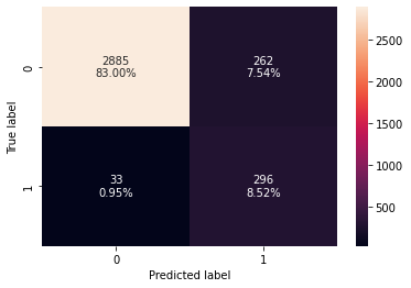
- True Negatives (TN): Correctly predicted that they do not have personal loan (2,885)
- True Positives (TP): Correctly predicted that they have personal loan (296)
- False Positives (FP): Incorrectly predicted that they have a personal loan (262 falsely predict positive Type I error)
- False Negatives (FN): Incorrectly predicted that they don’t have a personal loan (33 falsely predict negative Type II error)
Let’s review the score with the newly applied threshold.
#Checking model performance for this model
log_reg_model_train_perf_threshold_auc_roc = model_performance_classification_sklearn_with_threshold(lg, x_train, y_train, threshold=optimal_threshold_auc_roc)
print("Training performance:")
log_reg_model_train_perf_threshold_auc_roc
| Accuracy | Recall | Precision | F1 | |
| 0.915132 | 0.899696 | 0.530466 | 0.667418 |
This significantly improved our recall score but at the expense of our precision.
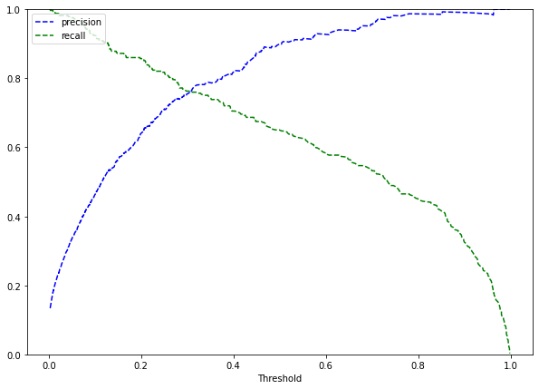
Model Using Optimal Threshold of .33
#Setting the threshold
optimal_threshold_curve = 0.33
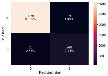
- True Negatives (TN): Correctly predicted that they do not have personal loan (3,078)
- True Positives (TP): Correctly predicted that they have personal loan (248)
- False Positives (FP): Incorrectly predicted that they have a personal loan (69 falsely predict positive Type I error)
- False Negatives (FN): Incorrectly predicted that they don’t have a personal loan (81 falsely predict negative Type II error)
Evaluating the score with the adjusted optimal threshold:
#Metrics with threshold set to 0.33
log_reg_model_train_perf_threshold_curve = model_performance_classification_sklearn_with_threshold(lg, x_train, y_train, threshold=optimal_threshold_curve)
print("Training performance:")
log_reg_model_train_perf_threshold_curve
| Accuracy | Recall | Precision | F1 | |
| 0.956847 | 0.753799 | 0.782334 | 0.767802 |
We successfully increased the precision, but the recall has now dropped. Since we are concerned about recall as that is the best measure for how well our model is predicting positive cases, we see that the model using the .12 threshold performed the best on our training data.
#Training performance comparison
models_train_comp_df = pd.concat(
    [
        log_reg_model_train_perf.T,
        log_reg_model_train_perf_threshold_auc_roc.T,
        log_reg_model_train_perf_threshold_curve.T,
    ],
    axis=1,
)
models_train_comp_df.columns = [
    "Logistic Regression sklearn",
    "Logistic Regression-0.12 Threshold",
    "Logistic Regression-0.33 Threshold",
]
print("Training performance comparison:")
models_train_comp_df
| Logistic Regression sklearn | Logistic Regression-0.12 Threshold | Logistic Regression-0.33 Threshold | |
| Accuracy | 0.959724 | 0.915132 | 0.956847 |
| Recall | 0.647416 | 0.899696 | 0.753799 |
| Precision | 0.898734 | 0.530466 | 0.782334 |
| F1 | 0.752650 | 0.667418 | 0.767802 |
We will now evaluate our model on the testing data.
Model Using sklearn
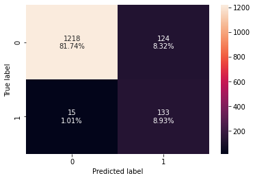
- True Negatives (TN): Correctly predicted that they do not have personal loan (1,218)
- True Positives (TP): Correctly predicted that they have personal loan (133)
- False Positives (FP): Incorrectly predicted that they have a personal loan (124 falsely predict positive Type I error)
- False Negatives (FN): Incorrectly predicted that they don’t have a personal loan (15 falsely predict negative Type II error)
#Metrics on test data
log_reg_model_test_perf = model_performance_classification_sklearn_with_threshold(lg, x_test, y_test)
print("Test set performance:")
log_reg_model_test_perf
| Accuracy | Recall | Precision | F1 | |
| 0.951678 | 0.608108 | 0.865385 | 0.714286 |
We will see if we can improve the recall scores using the optimal threshold. This has a really decent precision score however.
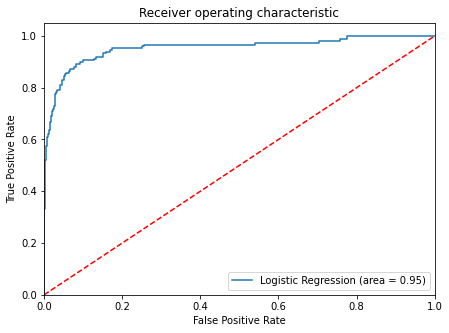
#Plot test data
logit_roc_auc_test = roc_auc_score(y_test, lg.predict_proba(x_test)[:, 1])
fpr, tpr, thresholds = roc_curve(y_test, lg.predict_proba(x_test)[:, 1])
plt.figure(figsize=(7, 5))
plt.plot(fpr, tpr, label="Logistic Regression (area = %0.2f)" % logit_roc_auc_test)
plt.plot([0, 1], [0, 1], "r--")
plt.xlim([0.0, 1.0])
plt.ylim([0.0, 1.05])
plt.xlabel("False Positive Rate")
plt.ylabel("True Positive Rate")
plt.title("Receiver operating characteristic")
plt.legend(loc="lower right")
plt.show()
Model Using Optimal Threshold of .12
#Creating confusion matrix on test with optimal threshold
confusion_matrix_sklearn_with_threshold(lg, x_test, y_test, threshold=optimal_threshold_auc_roc)

- True Negatives (TN): Correctly predicted that they do not have personal loan (1,218)
- True Positives (TP): Correctly predicted that they have personal loan (133)
- False Positives (FP): Incorrectly predicted that they have a personal loan (124 falsely predict positive Type I error)
- False Negatives (FN): Incorrectly predicted that they don’t have a personal loan (15 falsely predict negative Type II error)
Reviewing the metric scores using the optimal threshold set to 0.12, we see a very good recall score but a lower precision.
#Checking model performance for this model
log_reg_model_test_perf_threshold_auc_roc = model_performance_classification_sklearn_with_threshold(lg, x_test, y_test, threshold=optimal_threshold_auc_roc)
print("Test set performance:")
log_reg_model_test_perf_threshold_auc_roc
| Accuracy | Recall | Precision | F1 | |
| 0 | 0.906711 | 0.898649 | 0.51751 | 0.65679 |
Model Using 0.33 Threshold
Lastly, we will evaluate the testing data using a 0.33 threshold to see if we can improve these metrics any further.
#Creating confusion matrix with optimal threshold
confusion_matrix_sklearn_with_threshold(lg, x_test, y_test, threshold=optimal_threshold_curve)

- True Negatives (TN): Correctly predicted that they do not have personal loan (1,311)
- True Positives (TP): Correctly predicted that they have personal loan (105)
- False Positives (FP): Incorrectly predicted that they have a personal loan (31 falsely predict positive Type I error)
- False Negatives (FN): Incorrectly predicted that they don’t have a personal loan (43 falsely predict negative Type II error)
NOTE: Type I errors reduced to 31 from 124, but type II errors increased to 43 from 15.
#Checking model performance for this model
log_reg_model_test_perf_threshold_curve = model_performance_classification_sklearn_with_threshold(
    lg, x_test, y_test, threshold=optimal_threshold_curve
)
print("Test performance:")
log_reg_model_test_perf_threshold_curve
| Accuracy | Recall | Precision | F1 | |
| 0.950336 | 0.709459 | 0.772059 | 0.739437 |
e have successfully improved the precision. However, the recall score has significantly degraded. Additionally the model using the optimal threshold of 0.12 proves to be the strongest model.
#Testing performance
log_reg_model_test_perf_threshold_curve = model_performance_classification_sklearn_with_threshold(lg, x_test, y_test, threshold=optimal_threshold_curve)
log_reg_model_test_perf_threshold_curve
models_test_comp_df = pd.concat(
    [
        log_reg_model_test_perf.T,
        log_reg_model_test_perf_threshold_auc_roc.T,
        log_reg_model_test_perf_threshold_curve.T,
    ],
    axis=1,
)
models_test_comp_df.columns = [
    "Logistic Regression sklearn",
    "Logistic Regression-0.12 Threshold",
    "Logistic Regression-0.33 Threshold",
]
print("Test set performance comparison:")
models_test_comp_df
| Logistic Regression sklearn | Logistic Regression-0.12 Threshold | Logistic Regression-0.33 Threshold | |
| Accuracy | 0.951678 | 0.906711 | 0.950336 |
| Recall | 0.608108 | 0.898649 | 0.709459 |
| Precision | 0.865385 | 0.517510 | 0.772059 |
| F1 | 0.714286 | 0.656790 | 0.739437 |
We have successfully build a supervised learning classification model using logistic regression to help the marketing department to identify the potential customers who have a higher probability of purchasing a loan. Finding the optimal threshold of 0.12 had the strongest results with a recall of roughly 90% on both the testing and training data and had very strong accuracy scores. In a future post, we will expand this by using decision trees to evaluate how much stronger we can build this classification supervised learning model and provide the business some valuable insights.
